handnet
Digits on MNIST — the weights are 36 ASCII drawings
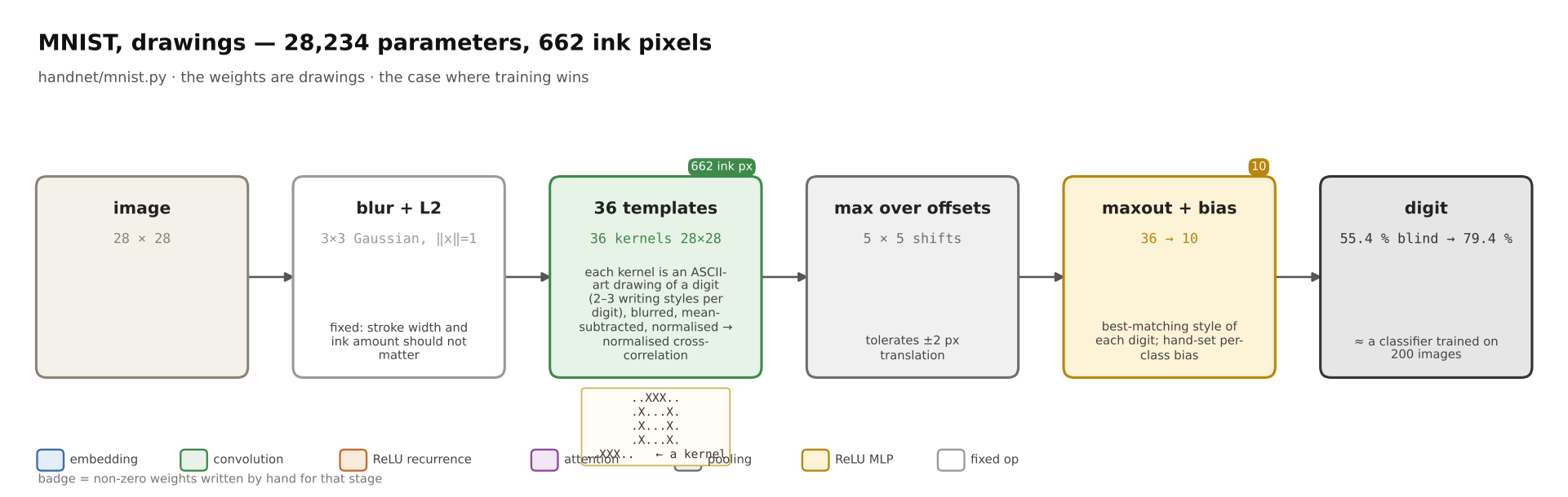
Source. 662 hand-drawn ink pixels, no training, numpy only. 55.4% blind, 79.4% after two revisions — what a trained classifier gets from about 200 labelled images. This is the case where hand-writing loses, and the confusion matrix explains why.
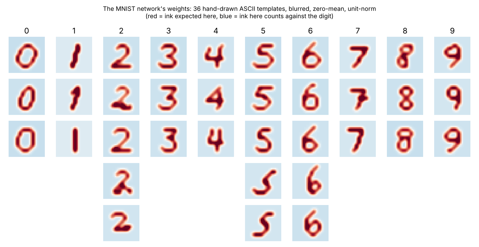
All 36 weights after the fixed expansion to 28×28 kernels. Red: ink expected. Blue: ink here is evidence against this digit. Each column is one class; rows are writing styles that a maxout layer chooses between.
Results
| Weights | Labels seen | Ink pixels drawn | Templates | Test accuracy |
|---|---|---|---|---|
| Hand-drawn | 0 | 544 | 28 | 55.4% |
| Hand-drawn, revision 1 | 500 (class means viewed) | 553 | 30 | 74.3% |
| Hand-drawn, revision 2 | 500 (error images viewed) | 662 | 36 | 79.4% |
| Trained logistic regression | 50 | — | — | 61.4% |
| Trained logistic regression | 100 | — | — | 71.5% |
| Trained MLP (64 hidden) | 100 | — | — | 71.8% |
| Trained logistic regression | 500 | — | — | 85.0% |
| Trained MLP (64 hidden) | 500 | — | — | 86.2% |
| Trained logistic regression | 10,000 | — | — | 90.9% |
| Trained MLP (64 hidden) | 10,000 | — | — | 95.4% |
MNIST test set, 10,000 images. Chance is 10%.
Architecture
image 28×28
  → 5×5 Gaussian blur (fixed) → zero-mean, unit-norm       ink amount should not matter
  → Conv2d(1 → 36, kernel 28×28, padding 3)                 36 hand-drawn templates
  → MaxPool over the 7×7 offsets                            tolerates ±3 px translation
  → Maxout 36 → 10 (best-matching style of each digit)
  → + per-class bias → argmax
A template is typed as 14×14 ASCII art. A fixed, parameter-free function turns it into a kernel: upsample ×2, widen the stroke to ~3 px with a cross-shaped 3×3 kernel, blur, subtract the mean, divide by the norm. Because the kernel is zero-mean and unit-norm the convolution output is a cosine similarity, and ink outside the stroke pulls the score down. That one detail was the difference between a 0 template that also fires on every 8 and one that does not.
0 (style 1)        1 (slanted, flag)   2 (loop base)       7 (with bar)
..............     ..............      ..............      ..............
..............     ..............      ..............      ..............
..............     ..............      ..............      ..............
......###.....     ........#.....      ......###.....      ..............
.....#...#....     .......##.....      .....#...#....      ....######....
....#.....#...     ......#.#.....      .........#....      .........#....
....#.....#...     ........#.....      ........#.....      ........#.....
...#......#...     .......#......      .......#......      .......####...
...#.....#....     .......#......      ......##......      ........#.....
...#.....#....     .......#......      .....#.##.....      .......#......
....#...#.....     ......#.......      ....#.#..##...      .......#......
.....###......     ......#.......      ....###...#...      ......#.......
..............     ..............      ..............      ..............
..............     ..............      ..............      ..............
The revisions
Revision 1 (+19 points). The blind drawings were systematically wrong: one grid row too high, upright instead of right-leaning, too wide. The model viewed the class-mean image of 500 labelled training digits next to its own templates and redrew all ten digits. This was the single most informative look at data in the whole project.
digit 7: class mean (500 train labels)   |  first blind template
   ..............                        |   ..............
   ..............                        |   ..............
   ..............                        |   ....+######...
   ..............                        |   .....+++++#+..
   ....+######...                        |   .........++...
   ...+#######...                        |   .........#+...
   ....##..+##...                        |   ........++....
   ........##+...                        |   ........#+....
   .......###....                        |   .......++.....
   .......##.....                        |   .......#+.....
   ......##+.....                        |   ......++......
   .....+#+......                        |   ......#+......
   ....+#++......                        |   ..............
   .....+........                        |   ..............
Revision 2 (+5 points). After revision 1 the weakest classes were 2, 5 and 6. The model viewed six misclassified training examples of each, drew two extra styles for each (a 2 with a looped base, a small high 2, a 5 without a top bar, a 6 with a long stem and a small low loop), widened the blur from 3×3 to 5×5 and the shift tolerance from ±2 to ±3 px.
Why this one loses
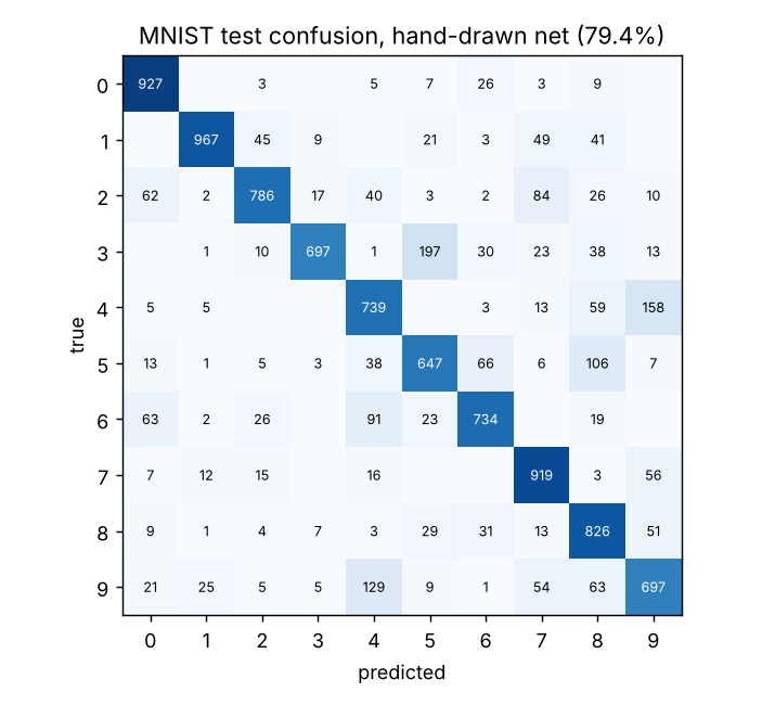
The big off-diagonal cells are 3→5 (197), 4→9 (158), 9→4 (129) and 5→8 (106). Those pairs differ in the presence of one small stroke — the top bar of a 5, whether a 9’s loop closes — which a whole-digit correlation barely notices against the shared bulk of the shape.
A trained linear classifier learns to put large weight on exactly those few discriminative pixels. A person drawing a prototype cannot know which pixels those are without looking at thousands of examples. The features that matter on MNIST are not nameable, so the “give every unit a job” step of the method has nothing to work with.
We also tried a part-based variant (hand-drawn stroke detectors into a hand-written 10×64 linear layer) and abandoned it: writing “how much does a horizontal stroke in the top-right speak for a 7” by hand for 640 cells is, on inspection, guessing.
Reproduce
python examples/mnist/eval_mnist.py                      # revision 2, 79.4%
python examples/mnist/handwritten_mnist_v2_rev1.py       # revision 1, 74.3%
python examples/mnist/handwritten_mnist_v1_blind.py      # blind, 55.4%
python examples/mnist/baselines_mnist.py                 # trained rows (scikit-learn)
python -m pytest -q tests/test_mnist.py
from handnet import mnist
X = mnist.load_idx("examples/mnist/data/t10k-images-idx3-ubyte.gz")
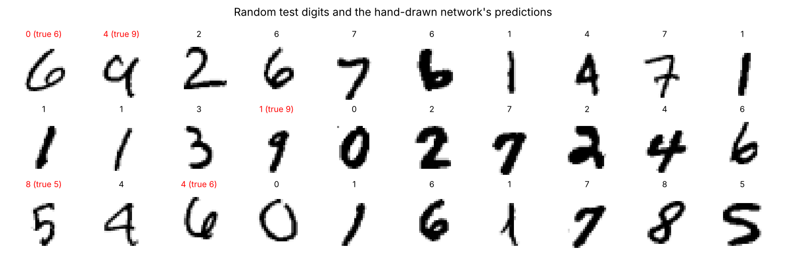
mnist.predict(X[:10]); mnist.explain(X[0])   # class scores = best template cosine per digit